The following tutorial describes how to analyze texts, by first generating linguistic annotations with a simple, single java program that bundles the abilities of several state-of-the-art NLP (Natural Language Processing) tools, and then accessing the annotations provided in a standardized output format for complex empirical analyses of text style and content in a scripting language. The workflows are based on a tool pipeline packaged from the DKPro framework for natural language processing into a single file, thus providing convenient access to many important DKPro features even for users with virtually no work experience with the framework. The example recipes further below describe how to use the pipeline’s output for advanced analytic procedures.
1. Setting Up the Pipeline
1.1. System Requirements
To run the pipeline properly, a system equipped with and able to handle at least 4 GB RAM is recommended. The following operating systems have been tested:
-
macOS (10.10 - 10.13)
-
Linux (Ubuntu 14.04 - 17.10)
-
Windows 7 - 10
Furthermore, the pipeline depends on an internet connection when running to download the models for the current configuration. It does not work offline!
1.2. Java Installation
The following step installs the base system requirements needed to run
DKPro Core pipelines on your machine. This needs to be performed only
once. Download and install the latest Java SE Runtime Environment (at least Java 1.8) from
the Oracle
Java Site, then follow the
installation
instructions for your operating system. You can check your current Java version by running java -version in your command line.
1.3. Pipeline Download
When the Java environment is prepared, you can download the latest binary. Select the file named ddw-0.4.7.zip and unpack it somewhere easily accessible. As a next step we need to navigate to this folder using the command line.
2. Running the Pipeline
2.1. Using the Command Line
The DKPro pipeline does not have a graphical user interface (GUI). Therefore you have to use the pipeline (both setting up and processing data) with the command prompt. In all versions of the Windows operating system, pressing the Windows key + "R" should launch the command prompt. Otherwise, the command prompt can be launched
-
in Windows 7 by clicking on the "Start"-button, type "command" in the search box and click on "Command Prompt"
-
in Windows 8 with a right-click on the “Start”-button, choosing “run", and typing “cmd” in the search box. Alternatively type "cmd" in the "Search".
-
in Windows 10 by typing "cmd.exe" into the search box on the taskbar and selecting the first option.
Navigate to the directory that contains the DKPro-pipeline. For example, if you are using windows and keeping your pipeline in folder named "DKPro" on drive "D:", by typing,
cd D:\DKPro
and press enter.
Alternatively the directory can be accessed instantly by holding Shift + right-clicking the folder needed and selecting "Open command window here".
2.2. Processing a Textfile
Now you can process a text file. How to test when you don’t have any
data? We’ve prepared a demonstration text that
can be downloaded and processed via the pipeline. You can compare your
output with this file.
If you receive an identical output DKPro pipeline works fine on your
computer. There are also a plenty of free texts available
from TextGrid Repository or Deutsches
Textarchiv. If you do not specify the -language parameter, the pipeline is prepared to analyze English input. For more details see further below.
To process data type the following command in the command prompt
java -Xmx4g -jar ddw-0.4.7.jar -input file.txt -output folder
and press Enter.
For example:
java -Xmx4g -jar ddw-0.4.7.jar -language de -input C:\EffiBriestKurz.txt -output D:\DKPro\Workspace
If your input and/or output file are located in the current directory you can type "." instead of the full input- and/or output-path. For example:
java -Xmx4g -jar ddw-0.4.7.jar -language de -input .\EffiBriestKurz.txt -output .
The pipeline will process your data and save the output as a .csv-File in the specified folder. If
File written, DONE
is shown on your command prompt everything has worked well. To see final
results check the output-file in your specified output folder.
Important Note: Depending on the configuration of your system and
the size of the input file processing may take some time, e.g. even
a test file of 630 words may easily take 1-2 minutes, even if 4 GB RAM
are allocated to the task.
2.3. File Reader
You can process either single files or also all files inside a directory. Patterns can be used to select specific files that should be processed.
2.3.1. Text Reader & XML Reader
The DARIAH-DKPro-Wrapper implements two base readers, one text reader and one XML-file reader. You can specify the reader that should be used with the -reader parameter. By default, the text reader is used. To use the XML reader, run the pipeline in the following way:
java -Xmx4g -jar ddw-0.4.7.jar -reader xml -input file.xml -output folder
The XML reader skips XML tags and processes only text which is inside the XML tags. The XPath to each tag is conserved and stored in the column SectionId in the output format.
2.3.2. Reading Directories
In case you want to process a collection of texts rather than just a single file, you can do that by providing a path to the -input option. If you run the pipeline in the following way:
java -Xmx4g -jar ddw-0.4.7.jar -input folder/With/Files/ -output folder
the pipeline will process all files with a .txt extension for the Text-reader. For the XML-reader, it will process all files with a .xml extension.
You can speficy also patterns to read in only certain files or files with certain extension. For example to read in only .tei with the XML reader, you must start the pipeline in the following way:
java -Xmx4g -jar ddw-0.4.7.jar -reader xml -input "folder/With/Files/*.tei" -output folder
Note: If you use patterns (i.e. paths containing an *), you must set it into quotation marks to prevent shell globbing.
To read all files in all subfolders, you can use a pattern like this:
java -Xmx4g -jar ddw-0.4.7.jar -input "folder/With/Subfolders/\**/*.txt" -output folder
This will read in all .txt files in all subfolders. Note that the subfolder path will not be maintained in the output folder.
2.4. Language
You can change the language by specifying the language parameter for the pipeline. Support for the following languages are included in the current version of the DARIAH-DKPro-Wrapper: German (de), English (en), Spanish (es), and French (fr). If you want to work with Bulgarian (bg), Danish (da), Estonian (et), Finnish (fi), Galician (gl), Latin (la), Mongolian (mn), Polish (pl), Russian (ru), Slovakian (sk) or Swahili (sw) input, you have to install TreeTagger first. To run the pipeline for German, execute the following command:
java -Xmx4g -jar ddw-0.4.7.jar -language de -input file.txt -output folder
2.5. Command Line Options
2.5.1. Help
The pipeline provides a help function that can be accessed on the command line with the "-help" option. Run java -jar ddw-{version}.jar -help to get an overview of the possible command line arguments:
 -config <path>     Config file
 -help              print this message
 -input <path>      Input path
 -language <lang>   Language code for input file (default: en)
 -output <path>     Output path
 -reader <reader>   Either text (default) or xml
 -resume            Already processed files will be skipped
The pipeline supports a resume function. By adding the -resume argument to the execution of the pipeline, all files that were previously processed and have an according .csv-file in the output folder will be skipped.
2.6. Troubleshooting
If there is no output in your output folder and your command prompt shows
Exception in thread "main" java.lang.OutOfMemoryError: Java heap space or The specified size exceeds the maximum representable size. Error: Could not create the Java Virtual Machine
you need to check the size of virtual memory. Depending on the maximum size of your RAM you should allocate 4GB or 6GB. The flag Xms specifies the initial memory allocation pool for a Java Virtual Machine (JVM). After adapting Windows' virtual memory type the following in the command prompt:
java –Xms -jar ddw-0.4.7.jar -input file.txt -output folder
and press enter.
For example, if you allocated 4GB then type:
java -Xms4g -jar ddw-0.4.7.jar -input EffiBriestKurz.txt -output D:\DKPro\Workspace
Note: Allocating too much virtual memory can slow down your system - 4GB or 6GB should be enough for most processing operations.
3. Available Components
As mentioned above, the pipeline contains a number of components
3.1. Segmentation
Segmentation is the task of dividing running text into units like sentences and words.
-
Word segmentation, also called tokenization, is the process of finding word boundaries - in its simplest form, by using the blanks in-between words as delimiters. However, there are languages that do not support this, such as Chinese or Japanese.
-
Sentence segmentation is the process of splitting text based on sentence limiting punctuation e.g. periods, question marks etc. Note that the periods are sometimes not the markers of sentence boundaries but the markers of abbreviations.
-
Besides, there are many other different segmentations on the basis of different purposes such as discourse segmentation (separating a document into a linear sequence of subtopics), Paragraph segmentation (which automatically break the text up into paragraphs) and so forth.
3.2. Part-of-Speech Tagging
Labeling every word and punctuation mark (token) in a text corpus with a predefined set of part-of-speech tags (standardized abbreviations) or other syntactic class markers, is called Part of Speech Tagging. Usually the output of a POS-Tagger will look like this (showing also DKPro’s CPOS column - a universal coarse grained tag set designed for the interoperability of components in different languages):
| Token | CPOS | POS |
|---|---|---|
Auf |
PP |
APPR |
einmal |
ADV |
ADV |
schien |
V |
VVFIN |
die |
ART |
ART |
Sonne |
NN |
NN |
durchzudringen |
V |
VVIZU |
Most tagging algorithms fall into one of two classes: rule-based taggers and probabilistic or stochastic taggers. Rule-based taggers generally involve a large database of hand-written disambiguation rules. Stochastic taggers generally resolve tagging ambiguities by using a training corpus to compute the probability of a given word having a given tag in a given context. Additionally there is an approach to tagging called the transformation-based tagger, or the Brill tagger, which shares features of both above tagging architectures.
3.3. Lemmatization
Mapping all different inflected word forms to one lemma is called lemmatization. It is related to stemming, an approach that tries to recognize derivational parts of a word to cut them off, leaving the stem as a result. In both cases, an amount of words are grouped together in a specific way. In stemming, the words are reduced to its stem. In lemmatization they are reduced to their common base lemma. The difference is, that a found stem would include every word containing the stem, but no other related words, as is the case with irregular verbs. Furthermore, the stem does not have to be a legit word, as long as it constitutes the common base morpheme. On the other hand, a lemma will most likely be the infinitive form of a verb or unmodified version of the word in question. Looking back to the example of stemming: Stemming of the words gone, going, and goes will not include the related term went, which would be the case after lemmatization.
3.4. Constituency and Dependency Parsing
Parsing is the main task behind breaking down a text into its more basic pieces and structures. A parser will take some input text and find specific structures, according to the preset rules, or syntax. Every conversion from one text-structure to another relies on parsing. If an algorithm takes a text and produces an output that contains the words with their corresponding part of speech (POS) tags, we can say, that the algorithm parsed the text finding words and adding POS information. Parsing is therefore the root of many kinds of linguistic analyses producing many sorts of structured output.
The idea of constituency is that groups of words may behave as a single unit or phrase, called a constituent such as the house, or a well-weathered three-story structure. The task of constituency parsing is to automatically find those words, which form the constituents. The final tree structure consists of final and non-final nodes. The final nodes are the words of the text that was parsed. The non-final nodes define the type of the phrase represented below the node.
In contrast, the notion of dependency foregrounds the words themselves and displays them as connected to each other by direct links. The structural center of the sentence is the verb to which every other word is (in)directly connected. Compared with the constituency form of representation, a dependency tree can be described as flat. The lack of phrase structure makes dependency grammars a good match for languages with free word order, such as Czech and Turkish.

.jpg)
3.5. Named Entity Recognition
Named entity recognition (NER) is a pre-processing step in most information extraction tasks. Named entity stands for the text block, which refers a name. NER describes the task of finding all names in one text and categorizing them based on their different types, such as persons, organizations or locations.
3.6. Semantic Role Labeling
Semantic role labeling (SRL, also: thematic role labeling, case role assignment) refers to a parsing approach that aims towards detecting all arguments of a verb. Ideally, it is able to assign appropriate semantic roles to its arguments (such as agent, patient, or instrument), thus preparing for a semantic interpretation of the sentence.
4. Configuring the Pipeline
4.1. Run the Full Pipeline
By default, the pipeline runs in a light mode, the memory and time intensive components for parsing and semantic role labeling are disabled.
If you like to use them, feel free to enable them in the default.properties or create a new .properties-File and pass the path to this file via the config-parameter.
4.2. Write Your Own Config File
The pipeline can be configurated via properties-files that are stored in the configs folder. In this folder you find a default.properties, the most basic configuration file. For the different supported languages, you can find further properties-files, for example default_de.properties for German, default_en.properties for English and so on.
If you like to write your own config file, just create your own .properties file. You have a range of possibilities to modify the pipeline for your purpose as you can see here.
For clarification have a look at line 3 to 13 in default.properties:
###################################
# Segmentation
###################################
useSegmenter = true # line 6
segmenter = de.tudarmstadt.ukp.dkpro.core.opennlp.OpenNlpSegmenter # line 7

# Possible values for segmenter:
# - de.tudarmstadt.ukp.dkpro.core.tokit.BreakIteratorSegmenter
# - de.tudarmstadt.ukp.dkpro.core.clearnlp.ClearNlpSegmenter
# - de.tudarmstadt.ukp.dkpro.core.opennlp.OpenNlpSegmenter (default)
# - de.tudarmstadt.ukp.dkpro.core.stanfordnlp.StanfordSegmenter
The component Segmentation is set to boolean true by default (line 6). If you want to disable Segmentation set useSegmenter to false. To use another toolkit than OpenNlpSegmenter (line 7), change the value of segmenter e.g. to de.tudarmstadt.ukp.dkpro.core.stanfordnlp.StanfordSegmenter for the StanfordSegmenter. A more specific modification with argument parameters is explained further below.
You can run the pipeline with your .properties-file by setting the command argument.
java -Xmx4g -jar ddw-0.4.7.jar -config /path/to/my/config/myconfigfile.properties -input file.txt -output folder
In case you store your myconfigfile.properties in the configs folder, you can run the pipeline via:
java -Xmx4g -jar ddw-0.4.7.jar -config myconfigfile.properties -input file.txt -output folder
You can split your config file into different parts and pass them all to the pipeline by seperating the paths using comma or semicolons. The pipeline examines all passed config files and derives the final configuration from all files. The config-file passed as last arguments has the highest priority, i.e. it can overwrite the values for all previous config files:
java -Xmx4g -jar ddw-0.4.7.jar -config myfile1.properties,myconfig2.properties,myfile3.properties -input file.txt -output folder
Note: The system always uses the default.properties and default_[langcode].properties as basic configuration files. All further config files are added on top of these files.
In case you like to use the full-version and also want to change the POS-tagger, you can run the pipeline in the following way:
java -Xmx4g -jar ddw-0.4.7.jar -config myFullVersion.properties,myPOSTagger.properties -input file.txt -output folder
In myPOSTagger.properties you just add the configuration for the different POS-tagger.
Note: The properties-files must use the ISO-8859-1 encoding. If you like to include UTF-8 characters, you must encode them using \u[HEXCode].
4.2.1. Understanding the Argument Parameter
A parameter is a special variable, consisting one or more arguments, provided to the subroutine. Most components of the DKPro pipeline can be equipped with arguments to specify for example the model that should be used. A list of possible arguments is available here in the column Constant Field or rather Value. Arguments are passed to the pipeline in a 3 tuple format:
-
The first tuple corresponds to the value of the Constant Field, e.g. writeDependency.
-
The second tuple declares the data type of the following tuple, e.g. boolean. As type you can use boolean, integer, and string.
-
The third tuple has to be a concrete data type value, e.g. false.
In the default.properties you can find the following line:
constituencyParserArguments = writeDependency,boolean,false
Here we specify the argument writeDependency with the boolean value false. This suggests, that no dependency annotations will be created.
4.3. Building Your Own
For creating your own pipeline the latest version of Java SDK (1.8 or higher), Eclipse (4.3.x), the Maven Integration for Eclipse (M2E) plugin and the DKPro Core ASL 1.8.0 or higher have to be installed on your computer. For further information see First Programming Steps with DKPro Core.
Some of the analysis components can be run with different models. For processing you can choose the component and the model that suits your interests the most from this list. For example, if you want to classify entities such as the names of persons, locations, expressions of times, organizations and so on there are two selectable components. StanfordNamedEntityRecognizer and OpenNlpNameFinder both are suitable for Named Entity Recognition. But if you are working with a German text StanfordNamedEntityRecognizer would be the better choice as you see in the list of models.
4.4. Using TreeTagger
Due to copyright issues, TreeTagger cannot directly be accessed from the DKPro repository. Instead, you have first to download and to install TreeTagger to able to use it with DKPro.
4.4.1. Installation
-
Go to the TreeTagger website
-
From the download section, download the correct tagger package, i.e. PC-Linux, OS X or Windows
-
Extract the .tar.gz and .zip archive, respectively
-
Create a new directory
tree-taggercontaining two foldersbinandlibon your hard drive, e.g.C:/tree-tagger/binandC:/tree-tagger/lib -
Copy the
tree-tagger/bin/tree-taggerfile from the previously downloaded archive to your recently created directorytree-taggerinto the folderbin
-
-
From the parameter file section, download the correct model. For the example below download Latin parameter file (latin-par-linux-3.2-utf8.bin.gz)
-
Unzip the file (e.g.
gunzip latin-par-linux-3.2-utf8.bin.gzor alternatively use a program like 7zip or WinRar) -
Copy the extracted file latin.par into the folder
libin your created directorytree-tagger
-
4.4.2. Configuration
After downloading the correct executable and correct model, we must configure our pipeline in order to be able to use TreeTagger. You can find an example configuration in the configs folder treetagger-example.properties:
posTagger =  de.tudarmstadt.ukp.dkpro.core.treetagger.TreeTaggerPosTagger
posTaggerArguments = executablePath,string,C:/tree-tagger/bin/tree-tagger.exe,\
	modelLocation,string,C:/tree-tagger/lib/latin.par,\
	modelEncoding,string,utf-8

# Treetagger adds lemmas, no need for an additional lemmatizer
useLemmatizer = false
Change the paths for the parameter executablePath and modelLocation to the correct paths on your machine. You can then use TreeTagger in your pipeline using the -config argument:
java -Xmx4g -jar ddw-0.4.7.jar -config treetagger-example.properties -language la -input file.txt -output folder
Check the output of the pipeline that TreeTagger is used. The output of your pipeline should look something like this:
POS-Tagger: true
POS-Tagger: class de.tudarmstadt.ukp.dkpro.core.treetagger.TreeTaggerPosTagger
POS-Tagger: executablePath, C:/tree-tagger/bin/tree-tagger.exe, modelLocation, C:/tree-tagger/lib/latin.par, modelEncoding, utf-8
5. Output Format
5.1. Specification
The wrapper’s output format is described in Fotis Jannidis, Stefan Pernes, Steffen Pielström, Isabella Reger, Nils Reimers, Thorsten Vitt: "DARIAH-DKPro-Wrapper Output Format (DOF) Specification". DARIAH-DE Working Papers Nr. 20. Göttingen: DARIAH-DE, 2016. URN: urn:nbn:de:gbv:7-dariah-2016-6-2.
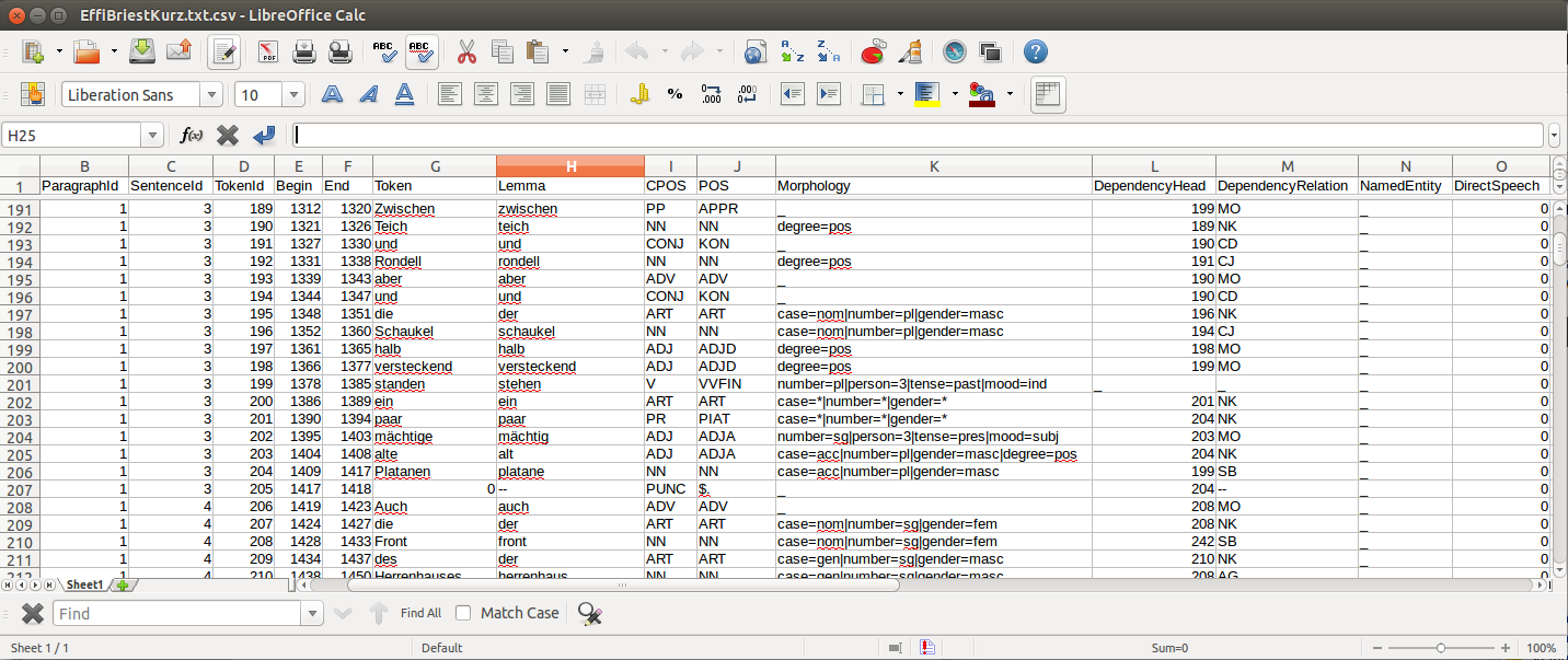
Example (from EffiBriestKurz.txt.csv):
5.2. Reading the Output
5.2.1. R
In R, a simple reader can be written as follows:
df = read.table("./data/EffiBriestKurz.txt.csv",    # or whatever file you want to read
                header = T,                         # first line as headers
                fill = T)                           # fill empty cells to avoid errors
5.2.2. Python
In Python, you can use the following code to ingest the output file.
import pandas as pd

import csv

df = pd.read_csv("EffiBriestKurz.txt.csv", sep="\t", quoting=csv.QUOTE_NONE)
5.3. Further Examples
You can also specify a subset of columns to use. Columns are addressed using their column names.
columns_input = ['SentenceId', 'TokenId', 'Token', 'CPOS']

df = df[columns_input]                                     # use only the selected columns
Use the pandas.DataFrame.groupby() method to easily access file contents. The following example shows how to retrieve a sentence.
sentences = df.groupby('SentenceId')                        # sort by sentence id

sent = sentences.get_group(10)                              # get sentence no. 10, returns a smaller dataframe
Using the same method, you can filter the entire file for a specific part-of-speech.
tags = df.groupby('CPOS')                                   # sort by CPOS values

adj = tags.get_group('ADJ')                                 # get all adjectives
Filtering for a specific value can also be done within a sentence.
nn = sent[sent['CPOS'] == 'NN'] # get nouns from the sentenceYou can use GroupBy-objects to process the entire file, e.g. in portions of sentences.
for sent_id, sent in sentences:                             # iterate through sentences

    for tok_id, tok, pos in zip(sent['TokenId'], sent['Token'], sent['CPOS']):  # go through each token in the sentence

        print(tok_id, tok, pos)
5.4. API
In addition to the examples above, an API (application program interface) will be provided, containing helper functions that simplify the retrieval of (combinations of) of features.
6. Example Recipe: Calculate Readability Measures in R
Extracting certain linguistic metrics using the output format of the NLP pipeline as a data frame in R or Python Pandas works straight forward. The following recipe is mainly aimed at demonstrating how to access, address, and use data in an R data frame. As already shown above, the output file can be loaded into the R environment with the following command:
df = read.table("PathToFile", header = T, fill = T)To compute, for example, the type token ratio (TTR) of the text, we take the column containing the tokens that can be addressed as 'df$Token'. We remove the punctuation by subsetting that vector formulating a logical condition that refers to the column containing the part-of-speech tags (df$Token[df$CPOS != "PUNC"]). The function unique() and length() allow us to generate a vector of unique types, and to measure the lengths of vectors.
types = length(unique(df$Token[df$CPOS != "PUNC"]))
tokens = length(df$Token[df$CPOS != "PUNC"])
TTR = types / tokens
Now, that we have computed the TTR, we can advance to slightly more complicated calculations in the same manner. Readability measures, a widely used class of linguistic metrics, are a simple means to estimate the difficulty of reading a text, e.g. to choose a suitable text for a reading exercise at school. We can easily calculate the such measures too. In this recipe we want to calculate both the so-called 'Automated Readability Index' or ARI and the LIX readability index from the output data frame in R. The ARI is calculated from the number of characters, the number of words, and the number of sentences. For computing the LIX we need the number of words, the number of periods, and the number of words longer than six characters.
The easiest step is to extract the number of sentences: The only thing you need to do is to find the highest sentence ID number using the function max() on the column containing the sentence IDs (df$sentenceId).
sentences = max(df$SentenceId, na.rm = T)To compute the number of words, we simply take the length of the Token column in the data frame (df$Token), again excluding all entries the POS-tagger has identified as punctuation symbols.
words = length(df$Token[df$CPOS != "PUNC"])The number of periods requires a somewhat more complicated excluding condition. Our POS tag set only marks punctuation in general, the LIX Readability Index specifically defines full stop period, colon, exclamation mark and question mark as periods. Hence, we want to exclude comma and semicolon from the selection. We will once more rely on the function length() to count elements. This time, we want to count only the elements tagged as punctuation (dfCPOS == "PUNC") and to exclude commas and semicolons.
periods = length(df$CPOS[df$CPOS == "PUNC" & df$Token != "," & df$Token != ";"])To calculate the remaining features, we begin by counting the characters in each word. The words themselves can be found in the column 'df$Token'. The function nchar() counts the characters in a string. The function lapply() can be used to apply nchar() upon each single element of df$Token. nchar() Can only be applied on character strings. To ensure that df$Token is of that type and has not accidentally interpreted as a factor when the data frame was loaded, we use the function as.character(), that can transform a factor into a vector of strings.
word_length = lapply(as.character(df$Token), nchar)As lapply() returns a list, we must convert the results into vector format (with unlist()), then we can get rid of the punctuation tokens.
word_length = unlist(word_length)
word_length = word_length[df$CPOS != "PUNC"]
Now that we have a vector at hand that contains the length of every single word in the text as a number, we can simply sum it up to calculate text length in characters.
characters = sum(word_length)And we can now compute the number long words, i.e. the number of words longer than six characters.
longwords = length(word_length[word_length > 6])Now all necessary features have been computed and stored in variables. To calculate the ARI for the text, we just need to put the feature values into the ARI formula,
ARI = 4.71 * (characters / words) + 0.5 * (words / sentences) - 21.43and into another formula for calculating the LIX.
LIX = (words / periods) + (100 * longwords / words)7. Example Recipe: Stylometric Analysis with the "Stylo" Package in R
In this recipe, we will demonstrate how to use the NLP pipeline’s output to explore different stylometrical aspects in a set of example texts using Stylo. The Stylo package is a popular tool written in R that provides a graphical interface to several functions for stylometrical analysis. Usually, Stylo takes a folder containing plain or xml text files as input. The user is then free to choose among different stylometrical procedures, e.g. PCA, and Burrows' Delta, and different kinds of features to analyze. Currently (in June 2015) available features are single words, word n-grams and character n-grams. In this recipe, it will be demonstrated how to use the output of our NLP pipeline to build sophisticated features for analysis in Stylo. In this example, two different feature types will replace the original words of the texts: the descriptive vocabulary, i.e. the adjectives and adverbs, and the abstract sentence structures in terms of n-grams of part-of-speech tags.
7.1. Example Corpus
The example set is a small collection of English short stories (the "small" and "short" aspects hopefully improving processing time in a way suitable for an example tutorial) written between 1889 and 1936 by four different authors: Rudyard Kipling, Arthur Conan Doyle, H. P. Lovecraft and Robert E. Howard. The texts are all public domain and available on Project Gutenberg, headers and metadata were removed from the plain text files before processing.
7.2. Preparing Descriptive Vocabulary and Part-of-Speech Tags
After running the NLP processing pipeline, the next step is to read out the relevant information from the CSV-files and store it in a form digestible for Stylo. Stylo processes input files from a folder named "corpus" in the working directory located within the current working directory.
The first thing to do is to set R’s working directory to your current working folder, i.e. the one where the CSV files are to be found. In R, the working directory can be changed using the "setwd()" command in the R console, like in
setwd("~/DKPro/")If you are uncertain about your current working directory, you can compute it by typing
getwd()The following R-code will extract the desired features from the CSV-files and store them in a Stylo-accessible way.
# Extract file names
files = list.files(pattern = "*.csv")

# Create directories
dir.create("dv/")
dir.create("pos/")
dir.create("dv/corpus/")
dir.create("pos/corpus/")

for(file in files)
{
  # Read file
  df = read.table(file, header = T, fill = T)

  # Prepare filename
  shortfile = sub(".csv", "", file)

  # Write Adjectives and Adverbes to analyse the author's inventaar of descriptive vocabulary
  dv = df$Lemma[df$CPOS == "ADJ" | df$CPOS == "ADV"]
  filename = paste("./dv/corpus/", shortfile, sep = "")
  write(paste(dv, collapse = " "), file = filename)

  # Write POS tags to compare sentence structure
  filename = paste("./pos/corpus/", shortfile, sep = "")
  write(paste(df$CPOS, collapse=" "), file = filename)
}
7.3. Using Stylo
If you have not installed the Stylo package yet, do that with the following command into the R console:
install.packages("stylo")Next, you can load the package with:
library(stylo)The workflow requires you at this point to decide on the particular analysis, either the descriptive vocabulary or the part-of-speech tag, you intend to start with. As Stylo only accepts a single "corpus" folder as input, you will have to do these separately. The order, however, depends on your preference (or curiosity) only. If you want to analyze the descriptive vocabulary, type:
setwd("./dv/")For working with part-of-speech tags, type:
setwd("./pos/")Once one of the folders is chosen, you can start Stylo by typing
stylo()into the R console. The interface will appear:
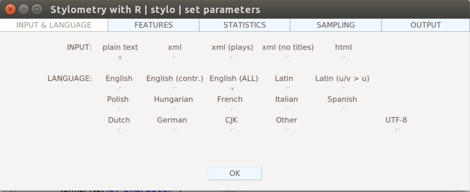
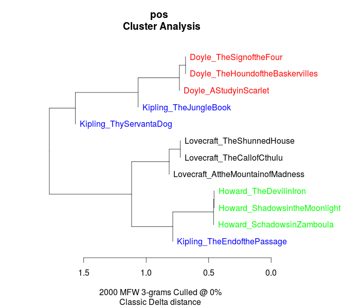
You can now, for example, run a cluster analysis in Stylo. Doing that with the unprocessed texts, yields the following result:
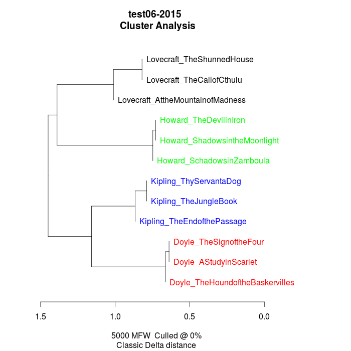
The authors are clearly separated, the British authors Doyle and Kipling are grouped together on one branch, the two Americans on the other.
Now, you can change into the folder with the descriptive vocabulary, and try the same procedure. With the example data set, we get the following result:
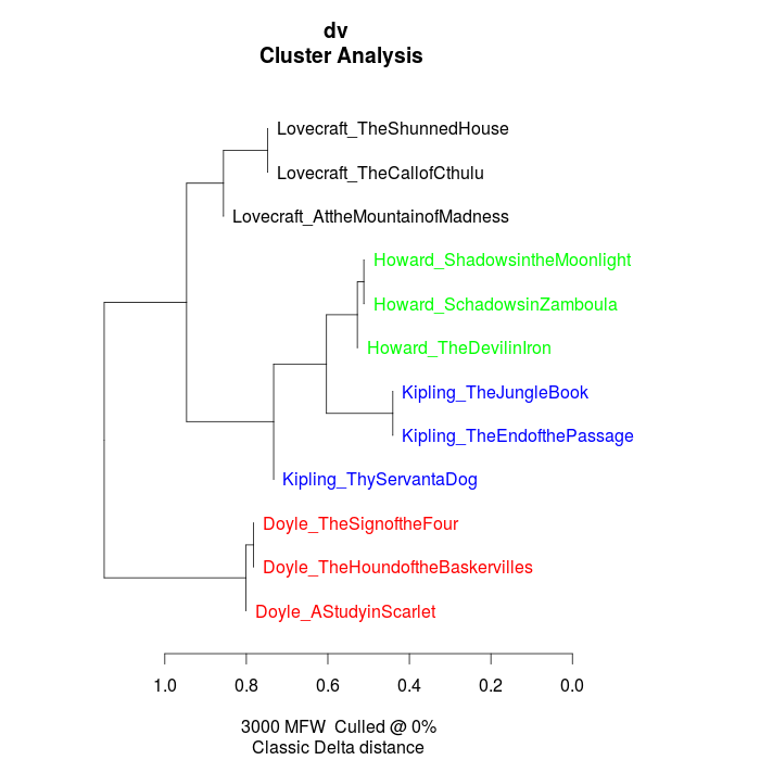
While text from the same authors still clustering together, it seems that, in contrary to their overall stylistic profile, Howard and Kipling are more similar to each other, than to the other investigated writers in terms of their preferred use of adjectives and adverbs.
Now, when changing into the folder containing the part-of-speech tags, it is important for gaining useful results to go to the "Features" tab in the Stylo interface and choose n-grams instead of single words as features. Our example data set, yields the following output, when using trigrams as features:
Interpreting the frequency trigrams of part-of-speech tags an approximation for the preference of certain sentence structures, three of the authors in the test set appear to be quite consistent in their individual syntax preferences, whereas the three texts the from Rudyard Kipling in our sample display a remarkable variability.
8. Example Recipe: Topic Modeling in Python
Topic modeling refers to a family of computational techniques that can be used to discover the main themes in a set of texts by statistically analyzing patterns of word usage. The term is often used synonymously with LDA (see Blei’s introductory paper), which is also the variant we will be working with in this tutorial. There have been written numerous introductions to topic modeling for humanists (e.g. [1] [2] [3]), which provide another level of detail regarding its technical and epistemic properties. Here it should just be pointed out that it is a bag-of-words approach purely based on word frequencies, which is unsupervised (it doesn’t have to be trained on any domain-specific dataset) and thus also works with literary and historical texts out of the box. However, as the algorithm was devised with summarizing news articles and other short text types in mind, its functioning is rather sensitive to text length. Also, depending on the research question, a rigorous selection process has shown to be fruitful, e.g. if you are not explicitly looking for the appearance of literary characters in certain semantic contexts, topics may become more informative when named entities are being excluded from the model.
We are using the Gensim package for Python (make sure v0.12.4 or higher is installed), but of course there are other well known LDA implementations, notably Mallett for Java and topicmodels for R.
You can find the complete, ready-to-run scripts for this recipe here.
8.1. Example Corpus
Any plain text or collection of texts can be used as input for topic modeling, however, this recipe is based on the pipeline’s CSV output for an improved feature selection process, e.g. controlling what should be included or excluded from the model. We will use the same collection of English short stories as in the last recipe, featuring works by Rudyard Kipling, Arthur Conan Doyle, H. P. Lovecraft, and Robert E. Howard.
8.2. Setting Up the Environment
The following code is designed to run with Python 3, which is recommended for its built-in Unicode capabilities and various other improvements. Assuming that you have Python (and its package manager pip) installed, issuing the following command at the command line will download and install the packages needed for this recipe:
pip3 install gensim pandas numpy pyLDAvisNote: In case pip install produces an error, try its predecessor easy_install. Not recommended on OS X, though, as the command defaults to the 2.7 Python installation that is shipped with OS X. Note: pyLDAvis is currently not available under Windows (as of 02/2016)
Also needed for this recipe is the widely used visualization package matplotlib (at least v1.5.1 or higher) for which installation directions are a bit different on each platform. If you are on a Debian based Linux system such as Ubuntu, you can use
sudo apt-get install python-matplotlibIf you are on OS X you can just use pip
pip3 install matplotlibFor installation on Windows (and other Linux systems), please have a look at matplotlib’s official documentation.
Now, for actually running this recipe, the most simplistic way would be to just start python and enter the code line by line, but it is highly recommended to look into IPython/Jupyter notebooks, if you like to work interactively. Most of the time however, you will want to put the code into a text file and make it a script that can be interpreted by Python. When naming the script, use the file extension .py - e.g. lda.py - and enter the following as its first line:
#!/usr/bin/env pythonThis takes care of finding the Python interpreter. Furthermore, on Unix systems the script needs to be made executable by typing chmod +x lda.py on the command line. On Windows systems everything should be handled automatically as of Python version 3.3.
If the following statements run without error, everything is installed correctly:
from gensim.corpora import MmCorpus, Dictionary
from gensim.models import LdaMulticore
import pandas as pd
import numpy as np
import os
import sys
import csv
These should be placed right after the first line, or, when working interactively, they are the first lines of the script.
Note: The model specified here is its parallelized version that uses all CPU cores to speed up training. For the single core version, just replace 'LdaMulticore' with 'LdaModel'.
8.3. Configuration Section
The following statements are so called 'constants' that reside in the global variable space of the script, being accessible to all functions and other sub-entities. This can be viewed as a configuration section, which we will use to set parameters for pre-processing and modeling.
# input
columns = ['ParagraphId', 'TokenId', 'Lemma', 'CPOS', 'NamedEntity']   # columns to read from csv file
pos_tags = ['ADJ', 'NN']                        # parts-of-speech to include into the model

# stopwords
stopwordlist = "stopwords.txt"                  # path to text file, e.g. stopwords.txt in the same directory as the script

# document size (in words)
#doc_size = 1000000 # set to arbitrarily large value to use original doc size
doc_size = 1000                                 # the document size for LDA commonly ranges from 500-2000 words
doc_split = 0                                   # uses the pipeline's ParagraphId to split text into documents, overrides doc_size - 1: on, 0: off

# model parameters, cf. https://radimrehurek.com/gensim/models/ldamodel.html
no_of_topics = 20                               # no. of topics to be generated
no_of_passes = 200                              # no. of lda iterations - usually, the more the better, but increases computing time

eval = 1                                        # perplexity estimation every n chunks - the smaller the better, but increases computing time
chunk = 10                                      # documents to process at once

alpha = "symmetric" # "symmetric", "asymmetric", "auto", or array (default: a symmetric 1.0/num_topics prior)
                                                # affects sparsity of the document-topic (theta) distribution


# custom alpha may increase topic coherence, but may also produce more topics with zero probability
#alpha = np.array([ 0.02, 0.02, 0.02, 0.03, 0.03, 0.03, 0.04, 0.04, 0.04, 0.05,
# 0.05, 0.04, 0.04, 0.04, 0.03, 0.03, 0.03, 0.02, 0.02, 0.02])

eta = None                                      # can be a number (int/float), an array, or None
                                                # affects topic-word (lambda) distribution - not necessarily beneficial to topic coherence
Note: Here, we are using the CPOS column, which takes its values from DKPro’s universal coarse-grained tag set (consisting of 13 tags: ADJ, ADV, ART, CARD, CONJ, N (NP, NN), O, PP, PR, V, PUNC). Alternatively, you can always use the POS column for a more fine grained selection. Currently the pipeline includes MatePosTagger, which produces output based on e.g. the Penn Tree Bank tag set for English and STTS for German. More information about DKPro components and the tag sets they are trained on can be found here.
8.4. Preparing the Data
As in many other machine learning applications, the amount of code needed to clean the data and to bring it into a form that can be processed far exceeds the actual modeling code (when using some kind of framework as it is the case here). What keeps the following code rather short, are the properties of the pipeline output format which make it easy to filter for feature combinations. As noted before - although in principle topic modeling works with completely unrestricted text - we want to be able to select certain word forms (based on their POS-tags) and match other restrictions (e.g. not to include named entities). Another thing we want to control is the size of text segments that get passed over to LDA as "documents" - as you experiment with different sizes you will notice that documents which are too large (novels as a whole) or too small (short scenes) both produce rather meaningless topics. A document size between 500 - 2000 words should yield acceptable results. Apart from producing arbitrary text segments of fixed size, we can also use the pipeline’s ParagraphId feature, which can be set to count paragraphs using a string pattern.
def preprocessing(path, columns, pos_tags, doc_size, doc_split, stopwordlist):
    docs = []
    doc_labels = []
    stopwords = ""

    print("reading files ...\n")

    try:
        with open(stopwordlist, 'r') as f: stopwords = f.read()
    except OSError:
        pass
    stopwords = sorted(set(stopwords.split("\n")))

    for file in os.listdir(path=path):
        if not file.startswith("."):
            filepath = path+"/"+file
            print(filepath)

            df = pd.read_csv(filepath, sep="\t", quoting=csv.QUOTE_NONE)
            df = df[columns]
            df = df.groupby('CPOS')

            doc = pd.DataFrame()
            for p in pos_tags:                          # collect only the specified parts-of-speech
                doc = doc.append(df.get_group(p))

            names = df.get_group('NP')['Lemma'].values.astype(str)  # add proper nouns to stopword list
            stopwords += names.tolist()

            # construct documents
            if doc_split:                               # size according to paragraph id
                doc = doc.groupby('ParagraphId')
                for para_id, para in doc:
                    docs.append(para['Lemma'].values.astype(str))
                    doc_labels.append(file.split(".")[0]+" #"+str(para_id))     # use filename + doc id as plot label
            else:                                       # size according to doc_size
                doc = doc.sort(columns='TokenId')
                i = 1
                while(doc_size < doc.shape[0]):
                    docs.append(doc[:doc_size]['Lemma'].values.astype(str))
                    doc_labels.append(file.split(".")[0]+" #"+str(i))
                    doc = doc.drop(doc.index[:doc_size])        # drop doc_size rows
                    i += 1
                docs.append(doc['Lemma'].values.astype(str))    # add the rest
                doc_labels.append(file.split(".")[0]+" #"+str(i))

    print("\nnormalizing and vectorizing ...\n")        # cf. https://radimrehurek.com/gensim/tut1.html

    texts = [[word for word in doc if word not in stopwords] for doc in docs]       # remove stopwords

    all_tokens = sum(texts, [])                                                     # remove words that appear only once
    tokens_once = set(word for word in set(all_tokens) if all_tokens.count(word) == 1)
    texts = [[word for word in text if word not in tokens_once] for text in texts]

    dictionary = Dictionary(texts)                      # vectorize
    corpus = [dictionary.doc2bow(text) for text in texts]

    return dictionary, corpus, doc_labels
It might be the case that filtering out named entities using information from the NamedEntity column still leaves too many unwanted names in the model. That can happen because NER components differ in performance for different languages and different types of text. An independently developed NER component trained on German 19th century novels will be included in a later version of the pipeline to address use cases like this. The following lines will add all named entities to the stopword list.
df = df.groupby('NamedEntity')

names = df.get_group('B-PER')['Lemma'].values.astype(str)

names += df.get_group('I-PER')['Lemma'].values.astype(str)

stopwords += names.tolist()
In the meanwhile, and as a more generic approach, we filter out all proper nouns (NP).
df = df.groupby('CPOS')

names = df.get_group('NP')['Lemma'].values.astype(str)

stopwords += names.tolist()
8.5. Fitting the Model
Next, we can put it all together. The following is the script’s entry point, which is usually placed at the bottom of every Python script. It checks for a command line argument, which should be a path. That path gets handed over to the preprocessing() function, which loads file after file and performs feature selection as well as vectorization of the data. The resulting dictionary and corpus objects are then used to create a LdaMulticore() model. Afterwards, the topics are displayed.
if len(sys.argv) < 2:
    print("usage: {0} [folder containing csv files]\n"
          "parameters are set inside the script.".format(sys.argv[0]))
    sys.exit(1)

path = sys.argv[1]
foldername = path.split("/")[-1]

dictionary, corpus, doc_labels = preprocessing(path, columns, pos_tags, doc_size, doc_split, stopwordlist)

print("fitting the model ...\n")

model = LdaMulticore(corpus=corpus, id2word=dictionary, num_topics=no_of_topics, passes=no_of_passes,
                 eval_every=eval, chunksize=chunk, alpha=alpha, eta=eta)

print(model, "\n")

topics = model.show_topics(num_topics=no_of_topics)

for item, i in zip(topics, enumerate(topics)):
    print("topic #"+str(i[0])+": "+str(item)+"\n")
For the example corpus this produces the following topics (shows the top 10 terms for each topic, the order of topics is random by default):
topic #0: 0.012*instant + 0.011*universe + 0.010*mad + 0.008*way + 0.008*everyone + 0.007*ship + 0.007*whilst + 0.007*other + 0.007*poor + 0.007*moment
topic #1: 0.008*world + 0.007*horror + 0.006*years + 0.006*body + 0.006*other + 0.006*terrible + 0.004*woman + 0.004*tree + 0.004*family + 0.004*baronet
topic #2: 0.009*corridor + 0.009*foot + 0.009*hand + 0.008*woman + 0.007*eyes + 0.007*lover + 0.007*floor + 0.006*chamber + 0.006*shape + 0.006*estate
topic #3: 0.012*point + 0.012*foot + 0.011*specimen + 0.011*inch + 0.009*print + 0.008*tube + 0.008*vegetable + 0.008*animal + 0.008*camp + 0.008*diameter
topic #4: 0.012*other + 0.012*way + 0.012*face + 0.010*case + 0.010*last + 0.010*eyes + 0.009*hand + 0.009*moor + 0.007*nothing + 0.006*anything
topic #5: 0.013*arms + 0.008*shape + 0.006*human + 0.005*tree + 0.005*lip + 0.005*neck + 0.005*face + 0.005*loam + 0.005*pave + 0.005*preferable
topic #6: 0.000*incoherent + 0.000*reality + 0.000*riches + 0.000*fearful + 0.000*neighbor + 0.000*oriental + 0.000*liking + 0.000*tentacle + 0.000*prize-fighter + 0.000*bristle
topic #7: 0.016*eyes + 0.012*poor + 0.011*anything + 0.010*hot + 0.009*punkah + 0.009*chap + 0.009*cooly + 0.008*face + 0.008*native + 0.006*sort
topic #8: 0.017*stain + 0.015*chemical + 0.012*test + 0.009*file + 0.009*rooms + 0.008*wagonette + 0.007*text + 0.007*eccentric + 0.007*fare + 0.006*misfortune
topic #9: 0.017*buffalo + 0.016*foot + 0.015*child + 0.015*herd + 0.014*things + 0.013*branch + 0.011*boy + 0.010*eyes + 0.010*moon + 0.009*skin
topic #10: 0.000*incoherent + 0.000*reality + 0.000*riches + 0.000*fearful + 0.000*neighbor + 0.000*oriental + 0.000*liking + 0.000*tentacle + 0.000*prize-fighter + 0.000*bristle
topic #11: 0.017*eyes + 0.013*tree + 0.013*foot + 0.009*hand + 0.008*cliff + 0.008*fire + 0.007*hands + 0.007*shoulder + 0.007*figure + 0.007*ruin
topic #12: 0.026*things + 0.020*dretful + 0.017*home + 0.016*while + 0.013*fine + 0.011*legs + 0.010*round + 0.010*afraid + 0.009*loud + 0.008*bit
topic #13: 0.000*incoherent + 0.000*reality + 0.000*riches + 0.000*fearful + 0.000*neighbor + 0.000*oriental + 0.000*liking + 0.000*tentacle + 0.000*prize-fighter + 0.000*bristle
topic #14: 0.013*desert + 0.008*palm + 0.008*human + 0.007*hand + 0.006*hut + 0.006*other + 0.006*lamp + 0.005*shadow + 0.005*eyes + 0.005*foot
topic #15: 0.009*case + 0.009*other + 0.008*family + 0.006*cellar + 0.005*manuscript + 0.005*record + 0.005*account + 0.005*much + 0.005*years + 0.005*interest
topic #16: 0.015*wind + 0.015*plane + 0.013*camp + 0.012*snow + 0.010*wireless + 0.010*world + 0.009*other + 0.009*antarctic + 0.008*whole + 0.008*seal
topic #17: 0.000*incoherent + 0.000*reality + 0.000*riches + 0.000*fearful + 0.000*neighbor + 0.000*oriental + 0.000*liking + 0.000*tentacle + 0.000*prize-fighter + 0.000*bristle
topic #18: 0.011*foot + 0.009*base + 0.008*plane + 0.008*world + 0.008*camp + 0.007*crew + 0.007*trip + 0.007*peak + 0.007*years + 0.006*unknown
topic #19: 0.003*cleanliness + 0.003*hawk-like + 0.003*luncheon + 0.000*readiness + 0.000*channels + 0.000*brigade + 0.000*enthusiast + 0.000*exactness + 0.000*edition + 0.000*politics
When you put everything together and do a test run, you will notice that producing an LDA model can take quite some time - if you have a lot of text to process, that might be something to do over night. Furthermore, as LDA is a generative and probabilistic model, its output is slightly different each time it is run (though, with a high number of iterations - see configuration section - results should be pretty stable).
Note: The configuration options implemented and discussed in this recipe will most likely have to be adjusted for use with another set of texts - be sure to experiment with different numbers of topics, iterations, document sizes, parts-of-speech to include, and if you’re feeling adventurous, also try different settings for the LDA hyperparameters - alpha and eta.
Note: If you want to know more about what’s happening under the hood, append the following to the import statements at the beginning of the file. Beware that Gensim’s logging produces a lot of detailed output.
import logging
logging.basicConfig(format='%(asctime)s : %(levelname)s : %(message)s', level=logging.INFO)
Finally, you can save calculated models to disk and load them afterwards, e.g. for experimenting with different visualizations. This last part of the script saves the model, corpus, and dictionary objects using Gensim’s save() function, as well as document labels and the topics themselves as text files.
print("saving ...\n")

if not os.path.exists("out"): os.makedirs("out")

with open("out/"+foldername+"_doclabels.txt", "w") as f:
    for item in doc_labels: f.write(item+"\n")

with open("out/"+foldername+"_topics.txt", "w") as f:
    for item, i in zip(topics, enumerate(topics)):
        f.write("topic #"+str(i[0])+": "+str(item)+"\n")

dictionary.save("out/"+foldername+".dict")
MmCorpus.serialize("out/"+foldername+".mm", corpus)
model.save("out/"+foldername+".lda")
8.6. Visualization Options
Each of the following visualizations is generated by its own Python script that is able to draw on contents and metadata of the LDA model using the save files generated by lda.py. The scripts expect a path to the generated model .lda file and that it is in the same directory as the other save files.
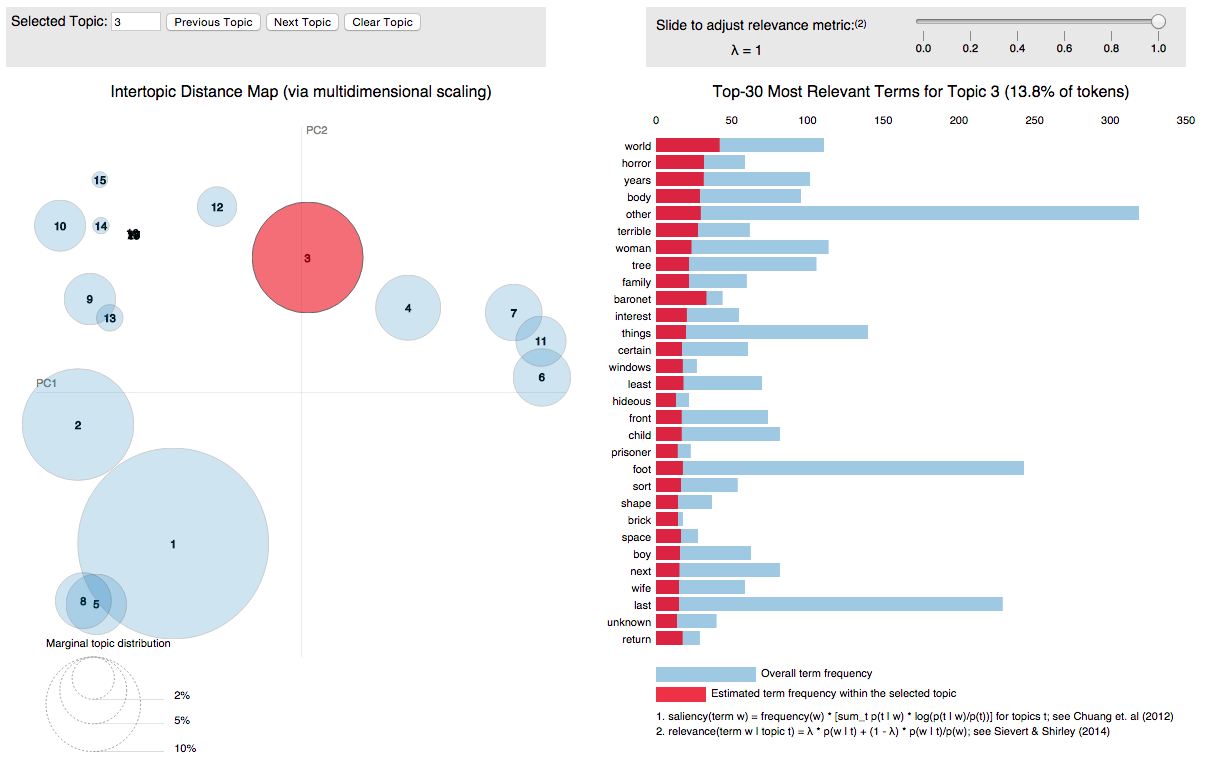
8.6.1. Interactive
[Source] This piece of code produces an interactive visualization of what the model has learned from the data. You can explore our example model by downloading this HTML file and opening it in a browser. The figure in the left column shows a projection of the inter-topic distances onto two dimensions, the barchart on the right shows the most useful terms for interpreting selected topic based on the 'relevance metric' slider. Basically, it allows for an interactive reranking and thus exploration of all terms connected to the topic, also those, which the model might have placed at the bottom. Another thing is that terms can be selected and in turn show how they are distributed on the map. The visualization package pyLDAvis has been described in this paper.
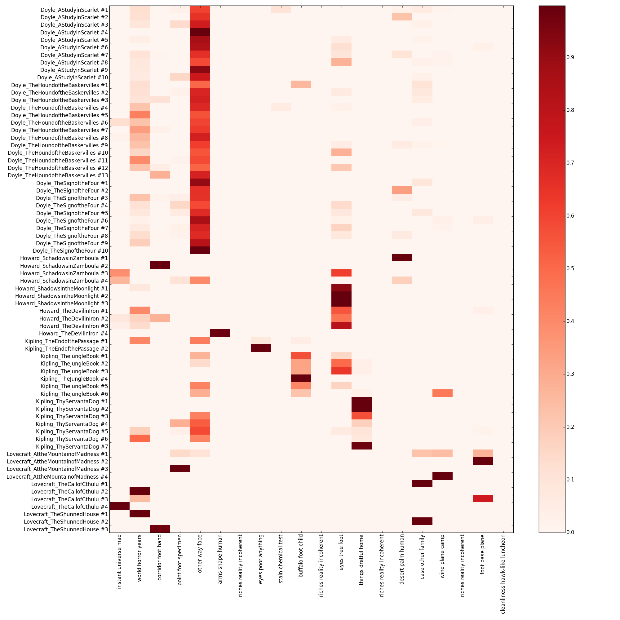
8.6.2. Heatmap
[Source] The heatmap option displays the kind of information that is probably most useful to literary scholars. Going beyond pure exploration, this visualization can be used to show thematic developments over a set of texts as well as a single text, akin to a dynamic topic model. What also becomes apparent here, is that some topics correlate highly with a specific author or group of authors, while other topics correlate highly with a specific text or group of texts. All in all, this displays two of LDA’s properties - its use as a distant reading tool that aims to get at text meaning, and its use as a provider of data that can be further used in computational analysis, such as document classification or authorship attribution. To get a feel for this visualization you can try e.g. building a number of models with varying document size (see configuration section in lda.py) - smaller document sizes 'zoom in' on the thematic development inside texts, while larger ones 'zoom out', up until there is only one row per document to display.
8.6.3. Network
[Source] For a more artistic presentation of a topic model, consider the following network graph that can be generated using a snippet from The Art of Literary Text Analysis by Stéfan Sinclair & Geoffrey Rockwell, namely the Graphing Topic Terms function, which produces the following graph:
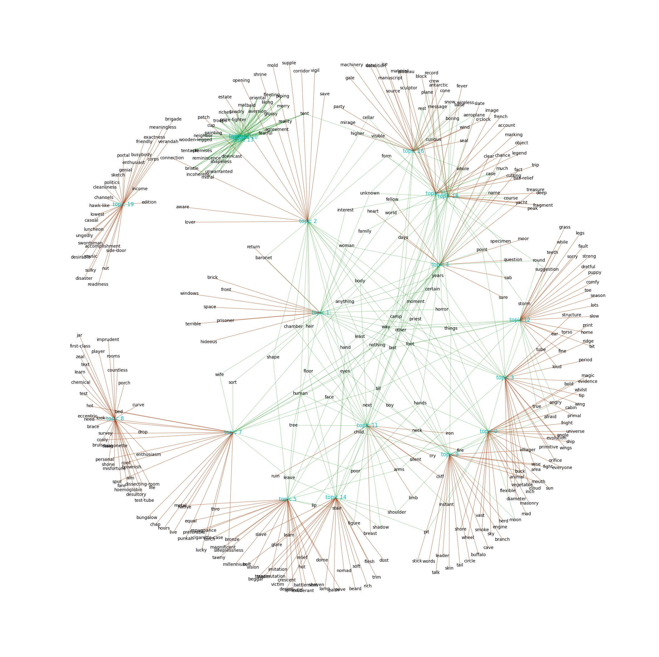
The graph shows the top 30 terms for each topic. Terms that are only connected to one topic are placed on the outside, while the terms that appear in more than one topic distribute themselves on the inside. In contrast to the interactive map example above, the topography of this network graph is not based on a distance measure but a product of the layout algorithm.
Note: You might want to try out various settings, depending on how many nodes you need to fit on the canvas. For this visualization the settings k=0.060, iterations=30 were passed to the nx.spring_layout() function.
9. Example Recipe: Stylometric Classification in Python
In this recipe, we will show how to implement a cross-genre stylometric classification system similar to the one proposed by van Halteren et al. in New Machine Learning Methods Demonstrate the Existence of a Human Stylome. In short, the authors propose a set of features and a classification algorithm based on the idea that everyone’s individual language form can be classified in terms of a 'stylome', as much as it can be for experienced writers. While we employ an ordinary Random Forest Classifier instead of the author’s own Weighted Probability Distribution Voting algorithm, we can show how to build a pairwise classification system that works genre-independently with an accuracy of around 0.70 using only the feature set.
You can find the complete, ready-to-run Python script on GitHub.
9.1. Example Corpus
The original corpus used in the paper is controlled for various factors and designed to make the classification task as hard as possible in order to substantiate the human stylome hypothesis. It consists of 72 Dutch texts by 8 authors, having roughly the same age and educational background. And it includes different text types: Each author was asked to produce three argumentative non-fiction texts, three descriptive non-fiction texts, and three fiction texts, each approximately 1,5 pages long. This led to a corpus controlled for register, genre and topic of the texts. It is suitable for training 72 models (for each possible pair of authors, based on eight texts each) and deriving a combined classification score.
Since we don’t have such a fine tuned corpus at hand, we decided to recreate part of it using freely available texts from Project Gutenberg. The example corpus provided here, consists of texts by two writers from roughly the same period, Heinrich von Kleist (1777–1811) and Franz Grillparzer (1791–1872). As it is the case for the original setup, this collection includes three prose texts, three plays, and three poems for each author. The filenames reflect their respective text types (although this information is not needed for the classification experiment) and indicate whether a longer text has been truncated ("Anfang"). Additionally, some poems had to be concatenated in order to arrive at a minimum text length of 300 words (labelled "Gedichte"). You can get the example corpus here.
9.2. Setting Up the Environment
Assuming you have Python installed, issuing the following command at the command line will download and install the packages needed for this recipe:
pip3 install pandas scikit-learnHave a look at the previous recipe setup for more detailed instructions. Now we can use the following import statements:
import pandas as pd
import numpy as np
import os, sys
from collections import Counter
from sklearn.feature_extraction import DictVectorizer
from sklearn.preprocessing import Imputer
from sklearn.ensemble import RandomForestClassifier
from sklearn.cross_validation import cross_val_score, ShuffleSplit
9.3. Feature Selection
The author’s approach to measuring a human stylome rests on the idea that any individual form can be classified as long as one looks for a large enough number of traits, consisting of both, vocabulary as well as syntactic features. This is also what the feature set in van Halteren et al. reflects:
   1. Current token
   2. Previous token
   3. Next token
   4. Concatenation of the wordclass tags of these three tokens (as
       assigned by an automatic WOTANlite tagger (van Halteren et al.., 2001)
   5. Concatenation of
       a. length of the sentence (in 7 classes: 1, 2, 3, 4, 5-10,11-20 or 21+
           tokens)
       b. position in the sentence (in 3 classes: first three tokens, last
           three tokens, other)
   6. Concatenation of
       a. part of speech of the current token, i.e. the initial part of the
           wordclass tag
       b. frequency of the current token in the text (in 5 classes: 1, 2-5,
           6-10,11-20 or 21+)
       c. number of blocks (consisting of 1/7th of the text) in which the
           current token is found (in 4 classes: 1, 2-3,4-6,7)
       d. distance in sentences to the previous occurrence of the current token
           (in 7 classes: NONE, SAME, 1, 2-3,4-7,8-15,16+)
Taken as a software specification this should prove a worthy test for the practicability of the CSV format. It translates into the following featureselect() function plus smaller functions to help with the calculation of specified classes:
def wordcount(wordlist):
    dict = {}
    for word in wordlist:
        if word not in dict: dict[word] = 1
        else: dict[word] += 1
    return dict

def token_in_textblock(text, token):        # returns number of blocks (consisting of 1/7th of the text)
    blocks = []                             # in which the current token is found, in 4 classes: 1, 2-3,4-6,7
    block_size = len(text)/7
    last = no_of_blocks = 0

    while last < len(text):
        blocks.append(text[int(last):int(last + block_size)])
        last += block_size

    for block in blocks:
        if token in block: no_of_blocks += 1

    if no_of_blocks == 1: occur_class = 1
    elif 2 <= no_of_blocks <= 3: occur_class = 2
    elif 4 <= no_of_blocks <= 6: occur_class = 3
    else: occur_class = 4

    return occur_class

def distance_to_previous(curr_tok_id, curr_sent_id, occurrences):
    # returns distance in sentences to the previous occurrence
    # of the current token (in 7 classes: NONE, SAME, 1, 2-3,4-7,8-15,16+

    occurrences = occurrences.reset_index()                             # add new index from 0 .. len(occurrences.index)

    current_key = occurrences[occurrences['TokenId'] == curr_tok_id].index[0]   # get row corresponding to curr_tok_id + its new index value

    if current_key > 0:                                                 # there is more than one && its not the first occurrence
        prev_sent_id = int(occurrences.iloc[current_key-1, 1])          # get previous sentence id based on that index

        dist = curr_sent_id - prev_sent_id

        if dist == 0: d_class = 2
        elif dist == 1: d_class = 3
        elif 2 <= dist <= 3: d_class = 4
        elif 4 <= dist <= 7: d_class = 5
        elif 8 <= dist <= 15: d_class = 6
        elif 16 <= dist: d_class = 7
    else:
        d_class = 1

    return d_class


def featureselect(text):
    columns = ['SentenceId', 'TokenId', 'Token', 'CPOS']
    columns_features = ['CurrToken', 'PrevToken', 'NextToken', 'TokenTags', 'LengthPosition', 'TagFreqOccur']

    csv = pd.read_csv(text, sep="\t")
    df = csv[columns]                               # create copy containing only the specified columns

    sent_max = df["SentenceId"].max()               # number of sentences in the text
    token_max = df["TokenId"].max()                 # number of tokens in the text

    text = list(df["Token"])
    word_freq = wordcount(text)                     # word frequencies

    features = pd.DataFrame(columns=columns_features, index=range(token_max+1))       # dataframe to hold the results

    for sent_id in range(sent_max+1):               # iterate through sentences
        sentence = df[df['SentenceId'] == sent_id]  # return rows corresponding to sent_id

        s_len = len(sentence.index)                 # length of the sentence
        if s_len == 1: s_class = 1                  # in 7 classes: 1, 2, 3, 4, 5-10,11-20 or 21+ tokens
        elif s_len == 2: s_class = 2
        elif s_len == 3: s_class = 3
        elif s_len == 4: s_class = 4
        elif 5 <= s_len <= 10: s_class = 5
        elif 11 <= s_len <= 20: s_class = 6
        elif 21 <= s_len: s_class = 7

        tok_count = 1
        for row in sentence.iterrows():
            tok_id = row[0]                         # row/dataframe index is the same as TokenId

            features.iat[tok_id, 0] = current_tok = row[1].get("Token")             # save current token
            tokentags = current_pos = row[1].get("CPOS")                            # get current pos tag

            if tok_id > 0:
                features.iat[tok_id, 1] = df.iloc[tok_id-1, 2]                      # save previous token
                tokentags += "-" + df.iloc[tok_id-1, 3]                             # get previous pos tag
            else:
                tokentags += "-NaN"

            if tok_id < token_max:
                features.iat[tok_id, 2] = df.iloc[tok_id+1, 2]                      # save next token
                tokentags += "-" + df.iloc[tok_id+1, 3]                             # get next pos tag
            else:
                tokentags += "-NaN"

            features.iat[tok_id, 3] = tokentags                         # save pos tags

            if tok_count <= 3: t_class = 1                              # position in the sentence
            elif (s_len-3) < tok_count <= s_len: t_class = 2            # in 3 classes: first three tokens, last three tokens, other
            else: t_class = 3

            features.iat[tok_id, 4] = str(s_class) + "-" + str(t_class) # save sentence length + token position

            tok_freq = word_freq[current_tok]                           # frequency of the current token in the text
            if tok_freq == 1: f_class = 1                               # in 5 classes: 1, 2-5, 6-10,11-20 or 21+
            elif 2 <= tok_freq <= 5: f_class = 2
            elif 6 <= tok_freq <= 10: f_class = 3
            elif 11 <= tok_freq <= 20: f_class = 4
            elif 21 <= tok_freq: f_class = 5

            block_occur = token_in_textblock(text, current_tok)

            occurrences = df[df['Token'] == current_tok]                # new dataframe containing all of curr_token's occurrences
            previous_distance = distance_to_previous(tok_id, sent_id, occurrences)

            features.iat[tok_id, 5] = current_pos + "-" + str(f_class) + "-" + str(block_occur) + "-" + str(previous_distance)

            tok_count += 1

    return features
The output is a DataFrame that looks like this:
           CurrToken       PrevToken       NextToken     TokenTags LengthPosition TagFreqOccur
0                Den             NaN     Mittelgrund    ART-NaN-NN            6-1    ART-2-1-1
1        Mittelgrund             Den          bilden      NN-ART-V            6-1     NN-1-1-1
2             bilden     Mittelgrund          Säulen       V-NN-NN            6-1      V-1-1-1
3             Säulen          bilden             mit       NN-V-PP            6-3     NN-1-1-1
4                mit          Säulen          weiten     PP-NN-ADJ            6-3     PP-3-3-1
5             weiten             mit  Zwischenräumen     ADJ-PP-NN            6-3    ADJ-1-1-1
6     Zwischenräumen          weiten               ,   NN-ADJ-PUNC            6-3     NN-1-1-1
7                  ,  Zwischenräumen             das   PUNC-NN-ART            6-3   PUNC-5-4-1
8                das               ,        Peristyl   ART-PUNC-NN            6-3    ART-3-3-1
9           Peristyl             das     bezeichnend    NN-ART-ADJ            6-2     NN-1-1-1
10       bezeichnend        Peristyl               .   ADJ-NN-PUNC            6-2    ADJ-1-1-1
11                 .     bezeichnend              Im   PUNC-ADJ-PP            6-2   PUNC-5-4-1
12                Im               .    Hintergrunde    PP-PUNC-NN            6-1     PP-2-2-1
13      Hintergrunde              Im             der     NN-PP-ART            6-1     NN-1-1-1
14               der    Hintergrunde          Tempel     ART-NN-NN            6-1    ART-5-4-1
15            Tempel             der               ,   NN-ART-PUNC            6-3     NN-3-3-1
16                 ,          Tempel              zu    PUNC-NN-PP            6-3   PUNC-5-4-3
17                zu               ,             dem    PP-PUNC-PR            6-3     PP-4-4-1
18               dem              zu         mehrere      PR-PP-PR            6-3     PR-3-3-1
19           mehrere             dem          Stufen      PR-PR-NN            6-3     PR-2-2-1
20            Stufen         mehrere     emporführen       NN-PR-V            6-2     NN-2-1-1
21       emporführen          Stufen               .     V-NN-PUNC            6-2      V-1-1-1
22                 .     emporführen            Nach     PUNC-V-PP            6-2   PUNC-5-4-3
23              Nach               .           vorne   PP-PUNC-ADV            6-1     PP-2-2-1
24             vorne            Nach               ,   ADV-PP-PUNC            6-1    ADV-1-1-1
25                 ,           vorne          rechts  PUNC-ADV-ADV            6-1   PUNC-5-4-3
26            rechts               ,             die  ADV-PUNC-ART            6-3    ADV-1-1-1
27               die          rechts          Statue    ART-ADV-NN            6-3    ART-5-4-1
28            Statue             die           Amors     NN-ART-NP            6-3     NN-1-1-1
29             Amors          Statue               ,    NP-NN-PUNC            6-3     NP-1-1-1
...              ...             ...             ...           ...            ...          ...
9.4. Preparing the Data
What we need to do now, is to gather this information in bulk and convert it into a form suitable for training, respectively testing a classifier. In order to achieve this, we write a function that loops over all CSV files in a directory and feeds them into featureselect() one by one. For each document, the resulting feature table gets trimmed down to n randomly selected observations (rows) and appended to a big DataFrame, which will become the input matrix X for the classification task. Simultaneously we build up a vector y, holding the corresponding author label for each observation. Next, the big DataFrame needs to be vectorized, e.g. converted from strings into numbers by use of a dictionary. This takes every distinct entry in the table and turns it into a column filled with 0’s and occasional 1’s for each time the encoded value shows up in a row. As one can imagine, the outcome is a table where the data is scattered among a lot of zeros, also called a sparse matrix. For the classifier to accept the data, we also need to make sure the matrix doesn’t contain missing values and use an imputer function that replaces NaN’s by the median of their respective rows.
def preprocessing(path, n):
    feats = []
    y = []

    print("processing files and randomly selecting {0} features each ...\n".format(n))

    for file in os.listdir(path=path):
        if not file.startswith("."):
            author = file.split("-")[0].replace("%20", " ")
            filepath = path+"/"+file
            print(filepath)

            for i in range(n): y.append(author)                     # add n labels to y

            with open(filepath, "r") as f:
                feat = featureselect(f)                             # perform feature selection
                rows = np.random.choice(feat.index.values, n)       # randomly select n observations
                feat_rand = feat.ix[rows]

                feats.append(feat_rand)
                f.close()

    data = pd.concat(feats, ignore_index=True)                      # merge into one dataframe

    print("\ndimensions of X: {0}".format(data.shape))
    print("dimensions of y: {0}\n".format(len(y)))

    print("vectorizing ...\n")

    vec = DictVectorizer(sparse=False)
    X = vec.fit_transform(data.T.to_dict().values())
    print("dimensions of X after vectorization: {0}\n".format(X.shape))

    imp = Imputer(missing_values='NaN', strategy='median', axis=0)    # replace NaN
    X = imp.fit_transform(X)

    return X, y, vec
9.5. Training and Evaluating the Classifier
Now, we can put it all together - first we check for two arguments, a folder containing CSV files for training and one file for testing the classifier. The folder gets passed on to the preprocessing() function, which returns the input matrix X, the label vector y, plus - as prerequisite for the prediction step later on - the dictionary used to vectorize X. Next, the RandomForestClassifier can be trained by providing the data and a number of parameters, here we use the number of trees in the model and the number of allowed concurrent processing threads. As specified in van Halteren et al., each model should be _"_trained on a collection of 11200 (2 authors x 8 training texts x 700 observations) feature vectors". The 8 training texts are part of a set of 9 texts for each author and comprise 3 different genres (see the corpus description). The number of observations can be traced back to properties of the originally used algorithm, but it is also a sensible default value for this adaption of the experiment.
Following training, an evaluation of the model using the scikit-learn cross validation function is performed. It is set up to use five randomly shuffled train and test sets in order to calculate a mean accuracy for the classifier.
n_obs = 700                                                         # no. of observations to select
n_trees = 30                                                        # no. of estimators in RandomForestClassifier

if len(sys.argv) < 3:
    print("usage: {0} [folder containing csv files for training] [csv file for testing]".format(sys.argv[0]))
    sys.exit(1)

# do feature selection, normalization, and vectorization
X, y, vec = preprocessing(sys.argv[1], n_obs)

# model training
print("training classifier ...\n")
clf = RandomForestClassifier(n_estimators=n_trees, n_jobs=-1).fit(X, y) # -1 sets n_jobs to the number of CPU cores
print(clf)

# evaluation
print("\nperforming cross validation (n_iter=5, test_size=0.125) ...")
cv = ShuffleSplit(X.shape[0], n_iter=5, test_size=0.125, random_state=4)
scores = cross_val_score(clf, X, y, cv=cv, n_jobs=-1)
print(scores)
print("mean accuracy: %0.2f (+/- %0.2f)\n" % (scores.mean(), scores.std() * 2))
Output:
processing files and randomly selecting 700 features each ...

train/Grillparzer%20-%20Das%20goldene%20Vließ%20(Anfang)%20(Drama).txt.csv
train/Grillparzer%20-%20Das%20Kloster%20bei%20Sendomir%20(Anfang)%20(Prosa).txt.csv
train/Grillparzer%20-%20Der%20arme%20Spielmann%20(Anfang)%20(Prosa).txt.csv
train/Grillparzer%20-%20Der%20Traum%20ein%20Leben%20(Anfang)%20(Drama).txt.csv
train/Grillparzer%20-%20Ein%20Erlebnis%20(Prosa).txt.csv
train/Grillparzer%20-%20Gedichte%201%20(Lyrik).txt.csv
train/Grillparzer%20-%20Gedichte%202%20(Lyrik).txt.csv
train/Grillparzer%20-%20Gedichte%203%20(Lyrik).txt.csv
train/von%20Kleist%20-%20Amphitryon%20(Anfang)%20(Drama).txt.csv
train/von%20Kleist%20-%20An%20Wilhelmine%20(Lyrik).txt.csv
train/von%20Kleist%20-%20Das%20Bettelweib%20von%20Locarno%20(Prosa).txt.csv
train/von%20Kleist%20-%20Das%20Erdbeben%20in%20Chili%20(Prosa).txt.csv
train/von%20Kleist%20-%20Das%20Käthchen%20von%20Heilbronn%20(Anfang)%20(Drama).txt.csv
train/von%20Kleist%20-%20Der%20Welt%20Lauf%20(Lyrik).txt.csv
train/von%20Kleist%20-%20Der%20zerbrochne%20Krug%20(Anfang)%20(Drama).txt.csv
train/von%20Kleist%20-%20Die%20beiden%20Tauben%20(Lyrik).txt.csv

dimensions of X: (11200, 6)
dimensions of y: 11200

vectorizing ...

dimensions of X after vectorization: (11200, 9692)

training classifier ...

RandomForestClassifier(bootstrap=True, class_weight=None, criterion='gini',
            max_depth=None, max_features='auto', max_leaf_nodes=None,
            min_samples_leaf=1, min_samples_split=2,
            min_weight_fraction_leaf=0.0, n_estimators=30, n_jobs=-1,
            oob_score=False, random_state=None, verbose=0,
            warm_start=False)

performing cross validation (n_iter=5, test_size=0.125) ...
[ 0.76214286  0.75928571  0.76714286  0.75142857  0.75785714]
mean accuracy: 0.76 (+/- 0.01)
9.6. Prediction Using the Classifier
Finally, we can use the trained classifier object to predict which author the text can be attributed to. The test text - which should be the 9th text from one author’s set and was not included in training the model - is sent through the same pre-processing steps as the other texts before. What matters here, is that we use the original classifier and DictVectorizer objects to vectorize and classify the test text.
Note: You can also decouple the prediction from the training part by using an already trained classifier object. See model persistence.
print("predicting author for {0} ...\n".format(sys.argv[2]))

# feature selection and preprocessing for testfile
with open(sys.argv[2], "r") as f:
    feat = featureselect(f)                             # perform feature selection
    rows = np.random.choice(feat.index.values, n_obs)       # randomly select n observations
    feat = feat.ix[rows]

print("dimensions of X_test: {0}".format(feat.shape))

X_test = vec.transform(feat.T.to_dict().values())       # vec must be the same DictVectorizer object as generated by preprocessing()

print("dimensions of X_test after vectorization: {0}\n".format(X_test.shape))

imp = Imputer(missing_values='NaN', strategy='median', axis=0)    # replace NaN
X_test = imp.fit_transform(X_test)

# prediction
y_pred = clf.predict(X_test)

c = Counter(y_pred)
c_key = list(c.keys())
c_val = list(c.values())
print(c_key[0], c_val[0]/(sum(c.values())/100), "% - ",
      c_key[1], c_val[1]/(sum(c.values())/100), "%")
Output:
predicting author for test/von%20Kleist%20-%20Der%20Findling%20(Prosa).txt.csv ...

dimensions of X_test: (700, 6)
dimensions of X_test after vectorization: (672, 9692)

von Kleist  77.52976190476191 % -  Grillparzer  22.470238095238095 %
Note: During vectorization, Python raises a warning because observations which cannot be found in the dictionary, have to be dropped. This is in fact how it should behave and if you want to suppress those warnings, you can append the following to the import statements:
import warnings
warnings.filterwarnings("ignore")
Discussion:
To wrap up, in this recipe we built a genre-independent 2-author-classifier using only the feature set from van Halteren et al.'s paper. While we did use neither the original algorithm, nor had a similarly controlled corpus at our disposal, the classifier displays an accuracy of around 0.70. Further tests will be needed to assess its cross-genre properties and accuracy in different settings. Furthermore, to really recreate the paper’s experimental setup, one would need to train classifiers for all possible pairs in a set of 8 authors and derive a combined classification score from that. All in all it is an encouraging start, though - the features as specified in the paper seem to be rather robust to different text types and might in fact show, that an individually measurable human stylome in writing exists. Apart from this experimental setting and prototypical authorship attribution problem, another possible application for such a high granularity classifier in the context of literary studies could be to measure stylistic differences within and in-between one author’s works (e.g. in order to reveal differences in narrators or focalizations).
We really encourage trying out different classifiers and parameters for this task. We have tried most which are included with scikit-learn and found that apart from Random Forests, the Decision Tree and the Gaussian Naive Bayes classifier perform pretty well. Let us know if you find other models and/or interesting parameter settings to work with and we will list them here.
10. Example Recipe: Network Visualization in Python
The following example attempts to show how to create a simple social network visualization of German poets by using text files extracted from Wikipedia. The Wikipedia API for Python is used to scrape the content from Wikipedia as plain text. With the help of the DARIAH-DKPro-Wrapper we gain access to the Named Entities (NE) in each file, compare them using basic Python programming and finally visualize them with the Python NetworkX and matplotlib packages. The basic assumption is that a connection between two authors exists if there is a certain amount of overlap in the Named Entities we extracted from their Wikipedia articles. Every author is represented by a node, a connection between two authors by an edge which is created when the number of overlaps passes a certain threshold.
You can find the ready-to-run scripts for this recipe here.
10.1. Setting Up the Environment
As explained in the example above you have to install three packages to realize this recipe. Issue the following command in the command line to download and install the needed packages:
pip3 install wikipedia
pip3 install networkx
Also make sure the package matplotlib is installed.
10.2. Crawling Wikipedia
The first part of the recipe is designed for interactive use. It is recommended to copy the following code into a text file and interpret it with Python through the command prompt. For more clearness the whole script is divided into small parts with explanations on what is going on in the single parts.
Use the following import statements in your first script after the first line:
import wikipedia
import re
In the following part we will create a new text file including a list of authors:
def create_authors(working_directory, wiki_page, wiki_section):
    """Gathers names from Wikipedia"""

    print("\nCreating authors.txt ...")
    with open(working_directory + "/authors.txt", "w", encoding='utf-8') as authors:
        full_content = wikipedia.page(wiki_page)
        selected_content = full_content.section(wiki_section)
        only_name = re.sub("[ \t\r\n\f]+[\(\[].*?[\]\)]","", selected_content)  # erases characters after full name
        authors.write(only_name)
        print(only_name)
As Wikipedia happens to consist of living documents, we provide a snapshot of a list of authors here.
Alternatively, you can create your own list of authors (make sure you use the exact name used by Wikipedia).
Output:
Creating authors.txt ...
Dietmar von Aist
Friedrich von Hausen
Heinrich von Rugge
Heinrich von Veldeke
Herger
Der von Kürenberg
Meinloh von Sevelingen
Rudolf von Fenis
Spervogel
To crawl the Wikipedia database with your determined authors list, add the following code to your script:
def crawl_wikipedia(authors_file, output_directory):
    """Crawls Wikipedia with authors.txt"""

    print("\nCrawling Wikipedia ...")
    with open(authors_file, "r", encoding="utf-8") as authors:
        for author in authors.read().splitlines():
            try:
                page_title = wikipedia.page(author)
                if page_title:
                    with open(output_directory + "/" + author + ".txt", "w", encoding='utf-8') as new_author:
                        new_author.write(page_title.content)
                        print(author + ": saved")

                else:
                    print("Error: Cannot create variable for wikipedia.page")

            except wikipedia.exceptions.DisambiguationError:
                pass
            except wikipedia.exceptions.HTTPTimeoutError:
                pass
            except wikipedia.exceptions.RedirectError:
                pass
            except wikipedia.exceptions.PageError:
                pass
Output:
Crawling Wikipedia ...
Dietmar von Aist: saved
Friedrich von Hausen: saved
Heinrich von Rugge: saved
Heinrich von Veldeke: saved
Herger: saved
Der von Kürenberg: saved
Meinloh von Sevelingen: saved
Rudolf von Fenis: saved
Spervogel: saved
Finally we are putting everything together. In case you have worked with the create_authors function use the following main() part:
def main(working_directory, output_directory, wiki_page, wiki_section):
    """
    :param working_directory: e.g. /users/networks
    :param output_directory: e.g. /users/networks/wikis
    :param wiki_page: e.g. "Liste deutschsprachiger Lyriker"
    :param wiki_section: e.g. "12. Jahrhundert"
    """

    wikipedia.set_lang("de")    # change language
    create_authors(working_directory, wiki_page, wiki_section)
    crawl_wikipedia(sys.argv[1] + "/authors.txt", output_directory)

if __name__ == "__main__":
    import sys
    main(sys.argv[1], sys.argv[2], sys.argv[3], sys.argv[4])
To run the script type the following command in your command line:
python3 script workingdirectory outputdirectory "wikipage" "wikisection"
and press Enter.
For example:
python3 /users/networks/crawler.py /users/networks /users/networks/wikis "Liste deutschsprachiger Lyriker" "12. Jahrhundert"
In case you already had a text file like authors.txt use the following main() part:
def main(authors_file, output_directory):
    """
    :param authors_file: e.g. /users/networks/my_own_file.txt
    :param output_directory: e.g. /users/networks/wikis
    """

    wikipedia.set_lang("de")    # change language
    crawl_wikipedia(authors_file, output_directory)

if __name__ == "__main__":
    import sys
    main(sys.argv[1], sys.argv[2])
To run the script type the following command in your command line:
python3 script authorsfile outputdirectory
and press Enter.
For example:
python3 /users/networks/crawler.py /users/networks/my_own_file.txt /users/networks/wikis
If everything worked fine you should have one text file authors.txt containing a list of names in your working directory. In your output folder there should be one text file for each author listed in authors.txt containing the specific Wikipedia page.
10.3. Using DKPro Wrapper and NetworkX to Visualize Networks
In the second part of the recipe you will analyze your previously created text files with the DKPro-Wrapper. How to process a collection of files in the same folder is explained further above. After creating a .csv file for each text file you use Python for further work on your files. Make sure you import the different modules first. Create the second (and last) script starting after the first line with:
import csv
from collections import defaultdict
import itertools
import glob
import os
import networkx as nx
import matplotlib.pyplot as plt
import re
The following function ingests the annotated file and extracts every NE. In the process first name and last name(s) or base name and extensions are merged. The .csv file marks first names and base names as B-PER and last names and extensions as I-PER. The function saves both B-PER and I-PER in a dictionary. Only B-PER or a B-PER followed by any combination of I-PER will be saved as one full name.
def ne_count(input_file):
    """Extracts only Named Entities"""

    ne_counter = defaultdict(int)
    with open(input_file, encoding='utf-8') as csv_file:
        read_csv = csv.DictReader(csv_file, delimiter='\t', quoting=csv.QUOTE_NONE)
        lemma = []

        for row in read_csv:
            if row['NamedEntity'] != "_" and row['CPOS'] != "PUNC":
                lemma.append(row['Lemma'])
            else:
                if lemma:
                    joined_lemma = ' '.join(lemma)
                    ne_counter[joined_lemma] += 1
                    lemma = []
    return ne_counter
This one is used to compare the dictionaries created above. It returns the number of matches which will be used to determine if an edge between two authors will be drawn:
def compare_ne_counter(ne_dict1, ne_dict2):
    """Compares two dictionaries"""

    weight = 0
    for key in ne_dict1.keys():
        if key in ne_dict2.keys():
            weight += 1
    print("this is the weight: " + str(weight))
    return weight
To label the nodes for the graph, this function extracts the names by removing the extensions of each author’s file name:
def extract_basename(file_path):
    """Extracts names from file names"""

    file_name_txt_csv = os.path.basename(file_path)
    file_name_txt = os.path.splitext(file_name_txt_csv)
    file_name = os.path.splitext(file_name_txt[0])
    return file_name[0]
Finally, creating the graph:
def create_graph(input_folder):
    """Creates graph including nodes and edges"""

    G = nx.Graph()
    file_list = glob.glob(input_folder)

    for item in file_list:
        G.add_node(extract_basename(item))

    for a, b in itertools.combinations(file_list, 2):
        weight = compare_ne_counter(ne_count(a), ne_count(b))
        if weight > 10:
            G.add_edge(extract_basename(a), extract_basename(b), {'weight': weight})
            # create edges a->b (weight)

    print("Number of nodes:", G.number_of_nodes(), "  Number of edges: ", G.number_of_edges())
    return G
Output:
this is the weight: 20
this is the weight: 11
this is the weight: 15
this is the weight: 7
this is the weight: 5
this is the weight: 9
this is the weight: 12
this is the weight: 18
this is the weight: 16
this is the weight: 10
this is the weight: 10
this is the weight: 14
this is the weight: 7
this is the weight: 8
this is the weight: 11
this is the weight: 9
this is the weight: 9
this is the weight: 9
this is the weight: 9
this is the weight: 8
this is the weight: 8
Number of nodes: 7   Number of edges:  8
The following code lastly is the main() function, which calls the previously defined functions after having the user select an input and output folder:
def main(input_folder, output_folder):
    """
    :param input_folder: e.g. /users/networks/csv
    :param output_folder: e.g. /users/networks
    """

    G = create_graph(input_folder + "/*")
    # If you want to create a circular graph, add '#' in front of every line of the following block,
    # erase the '#' of the three lines after 'Circular drawing', and run the script (again)
    pos = nx.spring_layout(G)
    nx.draw_networkx_labels(G, pos, font_size='8', font_color='r')
    nx.draw_networkx_edges(G, pos, alpha=0.1)
    plt.axis('off')
    plt.savefig(output_folder + "/graph.png")

    # Circular drawing:
    # nx.draw_circular(G, with_labels=True, alpha=0.3, font_size='8')
    # plt.axis('off')
    # plt.savefig(output_folder + "/circular.png")


if __name__ == "__main__":
    import sys
    main(sys.argv[1], sys.argv[2])
To run the script type the following command in your command line:
python3 script inputfolder outputfolder
and press Enter.
For example:
python3 /users/networks/graph.py /users/networks/csv /users/networks
Output:
Your output is a .png file and should look like one of these.
Poets of the 12th century:
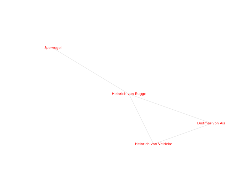
Poets of the 13th century:
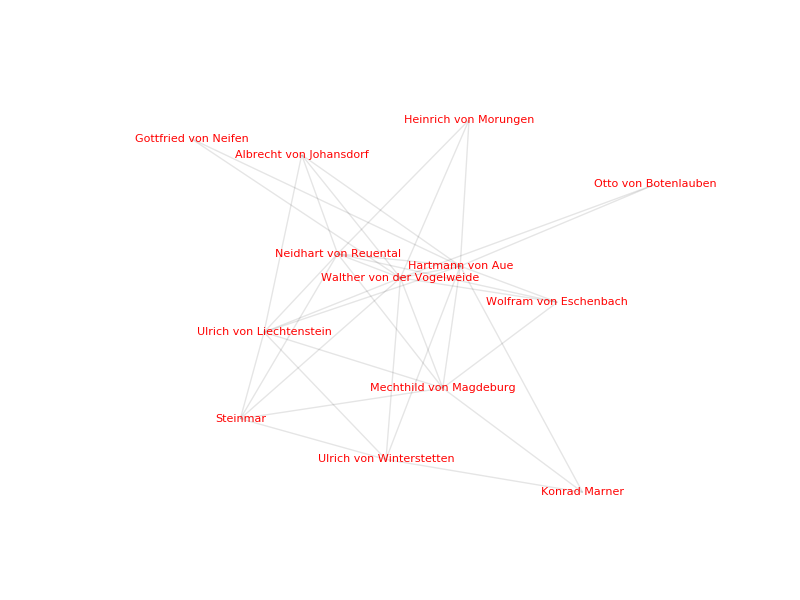
In case you decided to draw a circular graph:
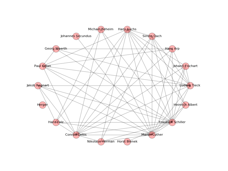
This recipe also works with other languages, e.g. English. You have to update the main part of the create_authors function and one possible output could look like this for "List of English-language poets" "A":
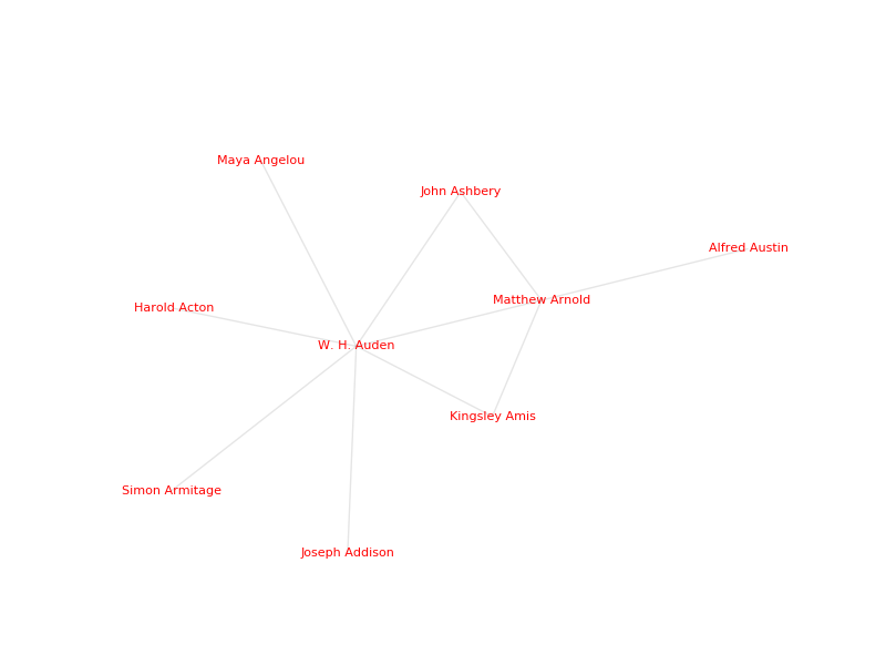
Discussion: In this recipe we created a visualization of an author’s social network using the output of the DARIAH-DKPro-Wrapper and two simple Python scripts to gain knowledge about the authors' relations. This is a great starting point for further research as the existing relations can now be examined more closely. The graphs might even hint at certain connections that have not been made yet. This kind of analysis therefore provides a groundwork and direction for further investigations on the topic.
11. About this Tutorial
Comments are welcome, as are reports of bugs and typos.
We would like to acknowledge the following individuals for their contributions to the continuing development of the tutorial:
-
Steffen Pielström
-
Stefan Pernes
-
Nils Reimers
-
Sina Bock
-
Philip Dürholt
-
Keli Du
-
Michael Huber
-
Severin Simmler
-
Thora Hagen
All materials are published under a Creative Commons Attribution 4.0 International license (CC-BY 4.0).
These tutorials have been developed with support from the DARIAH-DE initiative, the German branch of DARIAH-EU, the European Digital Research Infrastructure for the Arts and Humanities consortium. Funding has been provided by the German Federal Ministry for Research and Education (BMBF) under the identifier 01UG1110J.
![]()
![]()